Diffusion Policy almost Explained
To get a good grasp of diffusion policy, we need to understand diffusion models first. Here it goes.
 |
|---|
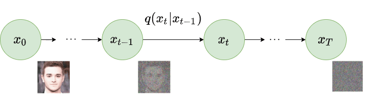
| Fig1 : The forward Markov chain for adding noise to the data. |
A denoising diffusion probabilistic model(DDPM) (1) uses two Markov chains, the forward diffusion process that converts data to noise and the reverse diffusion process that converts noise to data. The forward diffusion is usually handcrafted and the reverse diffusion is learned by a parameterized deep neural network.
Let us consider a data distribution $x_0 \sim q(x_0)$, the forward Markov chain generates a sequence of random variables $x_1, x_2, …, x_T$ using a transition kernel $q(x_t | x_{t-1})$. We can use the chain rule of probability and Markov property to write the joint distribution as $q(x_1, x_2, …, x_T)$ conditioned on $x_0$.
The formulae for the transition kernel is given by:
\[q(x_1, ..., x_T | x_0) = \prod_{t = 1}^T q(x_t | x_{t-1}) \tag{1}\]In DDPM the kernel is hancrafted generally and we use a Gaussian distribution for the transition kernel.
\[q(x_t | x_{t-1}) = \mathcal{N}(x_t; \sqrt{1 - \beta_t} x_{t-1}, \beta_t I) \tag{2}\]where $beta_t$ is a hyperparameter. $\beta_t \in (0, 1)$.
Now there is a long ass derivation to marginalise the joint distribution. For that use the following equation:
\[x_t = \sqrt{1-\beta} x_{t-1} + \sqrt{\beta} \mathcal{N} (0, \mathcal{I}) \tag{3}\]In this equation replace $x_{t-1}$ with $\sqrt{1-\beta} x_{t-2} + \sqrt{\beta} \mathcal{N} (0, \mathcal{I})$ and then $x_{t-2}$ with $\sqrt{1-\beta} x_{t-3} + \sqrt{\beta} \mathcal{N} (0, \mathcal{I})$ and so on till we reach $x_0$. This will take time to derive and we will get the following:
\[x_t = \sqrt{\alpha_t.\alpha_{t-1}...\alpha_1} x_0 + \sqrt{1-\alpha_t.\alpha_{t-1}...\alpha_1} \mathcal{N} (0, \mathcal{I}) \tag{4}\]where $\alpha_t = 1 - \beta_t$. So equation 4 can be written as:
\[x_t = \sqrt{\bar{\alpha}_t} x_0 + \sqrt{1-\bar{\alpha}_t} \mathcal{N} (0, \mathcal{I}) \tag{5}\]where $\bar{\alpha_t} = \prod_{i=1}^t \alpha_i$.
Hence we can write the joint distribution in the marginaslised form as:
\[q(x_t | x_0) = \mathcal{N}(x_t; \sqrt{\bar{\alpha}_t} x_0, (1-\bar{\alpha}_t) \mathcal{I}) \tag{6}\]Now given a a data point $x_0$ we can easily obtain $x_t$ by sampling a noise vector $\epsilon \sim \mathcal (0, \mathcal{I})$ from a Gaussian distribution and apply the follwing transformation : \(x_t = \sqrt{\bar{\alpha}_t} x_0 + \sqrt{1-\bar{\alpha}_t} \epsilon \tag{7}\)
The forward process is shown in the figure above where using the transition kernel an image is slowly converted to a pure Gaussian noise. Now we will discuss about the reverse Markov diffusion process where noise is gradually removed to generate a data point.
The reverse Markov chain is parameterised by a prior distribution $p(x_T) = \mathcal{N} (x_T; 0, \mathcal{I})$ and a learnable transition kernel $p_\theta(x_{t-1} | x_t)$ where $\theta$ is the learnable parameter of the deep neural network. The learnable transition kernel can expressed by the following equation:
\(p_\theta(x_{t-1} | x_t) = \mathcal{N}(x_{t-1}; \mu_\theta(x_t, t), \Sigma_\theta(x_t, t)) \tag{8}\)
In equation 8, $\mu_\theta(x_t, t)$ is the mean and $\Sigma_\theta(x_t, t)$ is the covariance of parameterised by the deep neural network. With the reverse Markov chain we can generate a data sample $x_0$ by first sampling a noise vector $x_T \sim p(x_T)$ and then iteratively sampling from the learnable transition kernel $x_{t-1} \sim p_\theta(x_{t-1} | x_t)$ till we reach $t = 1$. The idea is to train the Markov chain to match the actual reversal of the forward Markov chain. The deep neural network’s parameters $\theta$ are adjusted in such a wat that the joint distribution of the reverse Markov chain closely approximates the forward Markov chain. To match the forward Markov chain we need to minimise the KL divergence between the forward and reverse Markov chain. KL divergence is a measure of how different two probability distributions are. In our case the KL divergence between the forward and reverse Markov chain is given by:
The equation 9 can be further simplified to:
\[\mathcal{L} = -\mathbb{E}_{q(x_0,..x_T)} [log {p_{\theta} (x_0.. x_T)}] + constant \tag{10}\] \[\mathcal{L} = \mathbb{E}_{q(x_0,..x_T)} [ -log p(x_T) - \sum_{t = 1}^T log \frac{p_{\theta} (x_{t-1} | x_t)}{q(x_t | x_{t-1})}]+ constant \tag{11}\]The entire term before constant in equation 11 is the negative log likelihood of the reverse Markov chain which is called the variantional lower bound (VLB). Our aim is to minimise the negetive VLB i.e maximise the VLB. We formulate the loss function as mean squared error between the predicted and actual noise. An important the constant term is a lot of mathematical jargon which is not parameterised by theta and not trained by the optimizer so I ignored them. You can read it in the original paper (1).
The loss function is given by:
\(\mathcal{L}_{mse} = \mathbb{E}_{t \sim \mathcal{U} [1,T],x_0 \sim q(x_0), \epsilon \sim \mathcal{N}(0, \mathcal{I})}[ || \epsilon - \epsilon_\theta(x_t, t) ||^2] \tag{12}\)
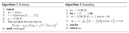
$x_t$ can be computed from $x_0$ and $\epsilon$ using equation 5. The deep learning network takes the noisy vector $x_t$ and the timestep $t$ as input and predicts the noise $\epsilon$ that was added to $x_0$ to get $x_t$. The timestep $t$ is sampled from a uniform distrbution. The optimizer trains the deep neural network $p_\theta$ to minimise the loss using the gradient descent algorithm.
During inference we can sample a pure Gaussian noise and then iteratively sample from the reverse Markov chain till we reach $t = 1$ to generate a data point.
 |
|---|
| Fig2 : The training and sampling(inference) method for DDPM |
Now lets get to Diffusion Policy, what we were here for. I took the diffusion policy image from the original paper by Chi et al. (2).
 |
|---|
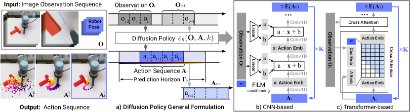
| Fig3 : Diffusion Policy architecture both Unet and transformer type. |
The authors have used diffusion models as a conditioned denoising process to generate robot motor behaviours. The observation (images from camera and proprioception data) from the robot’s environment has been processed to form in to condition vectors and then used to guide the diffusion to generate suitable motor signals for performing manipulation.
In the original paper by Chi et al.(2) the authors have used ResNet-18 to turn images from stationary cameras into observation embedding vectors. They replaced global average pooling with spatial softmax pooling previously used by Levine et al.(3)
and replaced batch normalisation layers with group normalisation for stable training of the ResNets.
For the noise scheduling the authors have found the use of squared cosine schedule to be best for their robotic tasks.
If the cosine scheduling function is defined as $f(t)$ which is a function of the diffusion step, then the alphas and betas of the
scheduler is defined as,
given that $f(t)$ is defined as,
\[f(t) = [cos(\frac{\frac{t}{T} + s}{1+s} \times \frac{\pi}{2})]^2\]where s is an offset, t is the timestep, T is the final timestep where the datapoint is a pure Gaussian. The values of $\beta_t$ are clipped to keep them less than 0.999 to prevent singularities at the end of the diffusion process when $t \rightarrow T$.
The problem formulation
The problem is formulated in such a way that the authors use a DDPM to approximate a conditional distribution $p(A_t | O_t)$. The actions are sampled from this conditional distribution which can be captured in the following way:
\[A_t^{k-1} = \alpha(A_t^k - \gamma\epsilon_\theta(O_t, A_t^k, k) + \mathcal{N}(0, \sigma^2\mathcal{I})) \tag{15}\]NOTE: In this notation k denotes the Markov chain timestep which was previously used as $t$ in equations 1-14, from equation 15 $k$ is similar to $t$ used before and $t$ refers to the timestep of the action sequence.
The loss is formulated using a mean squared error similar to equation 12.
\[\mathcal{L} = MSE(\epsilon^k, \epsilon_\theta(O_t, A_t^0 + \epsilon^k, k)) \tag{16}\]Training strategy
The steps to train such a diffusion policy is:
- Initialise the variance scheduler and calculate the alphas, betas and alpha cummulative products.
- Sample data sequence from demonstration dataset, select a random timestep for forward diffusion and use equation 7 to add noise to the action sequence using the variance schedule alphas. ($A_t^0 + \epsilon^k$)
- Use the sequence of observations. For example we have robot camera images in Fig 3. if we have camera images from 2 cameras say one is stationary and the other is attached to the robots wrist, pass them through two intialised resnets and concatenate them to get a common observation vector. In the CNN variant the author used FiLM conditioning (4) by Perez et al. where the observation vector is used to modulate the intermediate convolutional layers to guide the noise prediction. In the transformer variant of the architecture they have used minGPT (5) for the architecture where they used multiheaded cross attention to embed the observation with the noisy latents. Now pass the observation vector in whatever type of architecture you use (CNN or transformer) and get a noise prediction.
- Take MSE of the predicted noise and the actual pure Gaussian noise that was used in the second step while using equation 7. Take its gradient and backpropagate it using the optimizer.
- Do it again and again till you have trained the model for 3000 epochs (thats what the authors have done).
- After you are done training ensure saving the resnets and the main denoising architecture weights and state dictionary.
Inferencing strategy
Now to use the trained model to generate actions:
- Load the saved model into your GPU system. (CPU will do it very very slow)
- Collect the sequence of observation from cameras and pass it into the resnets and get the concatenated observation vector. Keep it.
- Now sample a Gaussian noise, using equation 15 use the observation vector to pass it into the denoising model for $k = T, T-1, …., 1, 0$ iterations to completely denoise the Gaussian to get the final action sequence $A_t^0$.
- Now comes an interesting part where the authors have taken $T_o$ observations at time (not diffusion step !!!!) $t$ to predict a long sequence denoted by $T_p$ called prediction horizon and executed only a part of it $T_a$ called action execution horizon. This has enabled the model to adapt to sudden changes in the observation and make the robot behave accordingly in case of failure to grasp an object or any kind of camera occlusion.
And thats how they turned a control problem into an elegant deep learning solution.
References
(1) Ho et al. Denoising diffusion probabilistic models , 2020
(2) Chi et al. Diffusion Policy : Visuomotor Policy Learning via Action Diffusion, 2023
(3) Levine et al. End-to-end training of deep visuomotor policies, 2015
(4) Perez et al. FiLM: visual reasoning with a general conditioning layer, 2017
(5) Github implementation by Andrej Karpathy for minGPT